Author: @BlazingKevin_ , the Researcher at Movemaker

In the cryptocurrency asset market, traders often encounter two typical problems: first, there is a significant gap between the highest bid price and the lowest ask price of the target trading token; second, after submitting a large market order, the asset price experiences drastic changes, causing the execution price to deviate significantly from expectations, resulting in high slippage costs. Both phenomena are caused by the same fundamental factor – insufficient market liquidity. The core market participants who systematically address this issue are market makers.

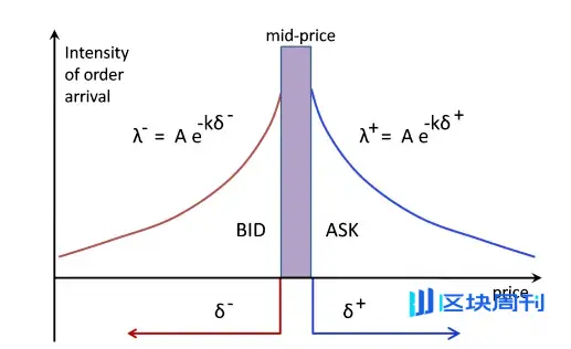
The precise definition of a market maker is a professional quantitative trading firm whose core business involves continuously and simultaneously submitting dense buy (Bid) and sell (Ask) quotes on the exchange's order book, centered around the current market price of the asset.

The fundamental function of their existence is to provide continuous liquidity to the market. Through bilateral quoting behavior, market makers directly narrow the bid-ask spread and increase the depth of the order book. This ensures that the buy and sell intentions of other traders can be matched instantly at any point in time, allowing transactions to be executed efficiently and at a fair price. As compensation for this service, market makers' profits come from the small spreads obtained from massive trading volumes, as well as the fee rebates paid by exchanges to incentivize liquidity provision.

The market conditions of 1011 have made the role of market makers the focus of market discussions. A key question arises when extreme price fluctuations occur: Did market makers passively trigger a chain liquidation, or did they proactively withdraw liquidity quotes in response to increased risk?

In order to analyze the behavioral patterns of market makers in similar situations, it is necessary to first understand the basic principles of their operation. This article aims to systematically answer the following core questions:

1. What is the business model that market makers rely on to make a profit?
2. What quantitative strategies will market makers adopt to achieve their business goals?
3. What risk control mechanisms will market makers activate when market volatility increases and potential risks arise?

Based on clarifying the above issues, we will be able to more clearly infer the behavioral logic and decision-making trajectory of market makers in the 1011 market.

Basic Profit Model for Market Makers

1.1 Core Profit Mechanism: Spread Capture and Liquidity Rebate

To understand the behavior of market makers in the market, it is essential to know their fundamental source of profit. Market makers provide continuous bid-ask quotes on the exchange order book (i.e., “making a market”); their profits are mainly composed of two parts: capturing the bid-ask spread and earning liquidity provision rebates from the exchange.

To illustrate this mechanism, we construct a simplified contract order book analysis model.

Assume there is an order book with the following distribution of buy and sell orders:

• Buy Orders (Bids): Concentrated at price levels of $1000.0, $999.9, $999.8, etc.
• Asks (Asks): Concentrated at price levels $1000.1, $1000.2, $1000.3, etc.

At the same time, we set the following market parameters:

• Transaction Fee: 0.02%
• Order Placement Rebate : 0.01%
• Minimum Price Increment : $0.1
• Current Spread (Spread): The difference between the best buy price ($1000.0) and the best sell price ($1000.1) is $0.1.

1.2 Transaction Process and Cost-Benefit Analysis

Now, let's break down the profit process of market makers through a complete trading cycle.

Step 1: Market Maker's Buy Order Passive Transaction ( Taker Sells )

Source: Movemaker

• Event: A trader (Taker) sells a contract at market price, and the order is matched with the best limit buy order on the order book, which is the buy order placed by the market maker at the $1000.0 price level.
• Nominal Cost: From the trading records, it appears that the market maker established a long position in a contract at a price of $1000.0.
• Effective Cost: However, since market makers are liquidity providers (Makers), this transaction not only incurs no fees but also earns a rebate of 0.01% from the exchange. In this case, the rebate amount is $1000.0 * 0.01% = $0.1. Therefore, the actual capital outflow (effective cost) for the market maker establishing this long position is: $1000.0 ( nominal cost ) - $0.1 ( rebate ) = $999.9.

Step 2: The market maker's sell order is executed passively (Taker Buys)

• Event: A trader (Taker) in the market buys a contract at the market price, and this order is executed against the best limit sell order on the order book, which is the sell order placed by the market maker at $1000.1. This action closes the long position established by the market maker in step one.
• Nominal Income: The trading record shows that the market maker sold at a price of $1000.1.
• Effective Income: Similarly, as a liquidity provider, the market maker receives a rebate of 0.01% on this sell trade, amounting to $1000.1 * 0.01% ≈ $0.1. Therefore, the actual capital inflow (effective income) for the market maker when closing the position is: $1000.1 ( nominal income ) + $0.1 ( rebate ) = $1000.2.

1.3 Conclusion: Composition of Real Profit

The total profit for the market maker per cycle of buying and selling is:

Total Revenue = Effective Income - Effective Cost = $1000.2 - $999.9 = $0.3

It can be seen that the real profit of market makers is not just the nominal spread of $0.1 visible on the order book. The true composition of their profit is:

Real Profit = Nominal Price Difference + Buy Order Rebate + Sell Order Rebate

$0.3=$0.1+$0.1+$0.1

This pattern of accumulating small profits through countless repetitions of the above process in high-frequency trading constitutes the most fundamental and core profit model of market-making business.

Dynamic Strategies and Risk Exposure of Market Makers

2.1 Challenges Faced by the Profit Model: Directional Price Movements

The aforementioned basic profit model is predicated on the premise that market prices fluctuate within a narrow range. However, when the market experiences a clear unilateral directional movement, this model will face severe challenges and expose market makers directly to a core risk - adverse selection risk.

Adverse selection refers to a situation where informed traders selectively transact at prices offered by market makers that have not yet been updated, which are at the “wrong” price, when new information enters the market and causes a change in the fair value of the asset, resulting in market makers accumulating unfavorable positions.

2.2 Scenario Analysis: Strategies for Responding to Price Declines

To illustrate specifically, we continue with the previous analytical model and introduce a market event: the fair price of the asset rapidly dropped from $1000 to $998.0.

Suppose the market maker only holds a long contract established in a previous transaction, with an effective cost of $999.9. If the market maker takes no action, the buy orders placed around $1000.0 will present a risk-free profit opportunity for arbitrageurs. Therefore, once a directional price movement is detected, the market maker must respond immediately, with the primary action being to actively withdraw all buy orders close to the old market price.

At this time, market makers face a strategic choice, mainly with the following three response options:

• Option 1: Close Position Immediately to Realize Loss The market maker can choose to sell the held long contracts immediately at the market price. Assuming the transaction is executed at $998.0, the market maker will need to pay a taker fee of 0.02%.

Loss = ( effective cost - exit price ) + taker fee

Loss = ($999.9 − $998.0) + ($998.0 × 0.02%) ≈ $1.9 + $0.2 = $2.1

The purpose of this plan is to quickly eliminate risk exposure, but it will immediately result in a certain loss.

• Option 2: Adjust the quote to seek a better exit price Market makers can lower their sell one quote to a new market fair price, for example $998.1. If the sell order is executed, the market maker will receive a rebate as the maker.

Loss = ( Effective Cost − Exit Price ) − Order Rebate

Loss = ($999.9 − $998.1) − ($998.1 × 0.01%) ≈ $1.8 − $0.1 = $1.7

This plan aims to exit positions with smaller losses.

• Option 3: Expand the Price Spread and Manage Existing Positions Market makers can adopt an asymmetric quoting strategy: adjust the sell price to a relatively unappealing level (e.g., $998.8), while placing new buy orders at lower price levels (e.g., $998.0 and $997.9). The goal of this strategy is to manage and reduce the average cost of existing positions through subsequent trades.

2.3 Strategy Execution and Inventory Risk Management

Assuming under the “single market maker” market structure, due to its absolute pricing power, the market maker is likely to choose option three to avoid realizing a loss immediately. In this option, the sell order price ($998.8) is far higher than the fair price ($998.0), which results in a lower probability of execution. Conversely, the buy order that is closer to the fair price ($998.0) is more likely to be executed by sellers in the market.

Step 1: Lower the average cost by increasing holdings

• Event: The buy order placed by the market maker at $998.0 has been executed.
• Effective cost of new position: $998.0 - (998.0×0.01%)≈$997.9
• Updated Total Position: The market maker now holds two long contracts with a total effective cost of 999.9+$997.9=$1997.8.
• Updated Average Cost: $1997.8 / 2 = $998.9

Step 2: Adjust Quotation Based on New Costs

Through the above operations, the market maker successfully lowered the breakeven point of its long position from $999.9 to $998.9. Based on this lower cost basis, the market maker can now more aggressively seek selling opportunities. For example, it can significantly lower the sell quote from $998.8 to $998.9, achieving breakeven while narrowing the spread from $1.8 ($999.8 - $998.0) to $0.8 ($998.8 - $998.0) to attract buyers.

2.4 Limitations of Strategies and Exposure to Risks

However, this strategy of averaging down through increased holdings has obvious limitations. If the price continues to drop, for example, plummeting from $1000 to $900, the market makers will be forced to keep increasing their holdings under continuous losses, which will sharply amplify their inventory risk. At that time, continuing to widen the spread will lead to a complete halt in trading, creating a vicious cycle, ultimately forcing them to liquidate at a significant loss.

This raises a deeper question: how do market makers define and quantify risk? What core factors are related to different levels of risk? The answers to these questions are key to understanding their behavior in extreme markets.

Core Risk Factors and Dynamic Strategy Development

The profit model of market makers essentially involves taking on specific risks in exchange for returns. Their losses primarily stem from significant short-term deviations in asset prices that are unfavorable to their inventory positions. Therefore, understanding their risk management framework is key to analyzing their behavioral logic.

3.1 Identification and Quantification of Core Risks

The risks faced by market makers can be summarized as two interrelated core factors:

1. Market Volatility: This is the primary risk factor. An increase in volatility means that both the likelihood and magnitude of price deviations from the current mean are increasing, directly threatening the inventory value of market makers.
2. Speed of Mean Reversion: This is the second key factor. After a price deviation occurs, whether it can return to equilibrium levels in a short time determines whether the market maker can ultimately profit by averaging costs or will fall into continuous losses.

A key observable indicator for judging the possibility of mean reversion is trading volume. In the article “A Review of Intensified Market Discrepancies: Does the Rebound Shift to a Reversal, or is it a Second Distribution in a Downtrend?” published by the author on April 22 this year, the theory of marbles in the order book was mentioned. Limit orders at different prices form a glass layer of uneven thickness based on the order volume, and a fluctuating market is like a marble. We can consider the limit orders at different price levels in the order book as a “liquidity absorption layer” with varying thickness.

Short-term price fluctuations in the market can be viewed as a marble of shock force. In a low trading volume environment, the shock force is weaker, and prices are usually confined to narrow movements between the most dense liquidity layers. In a high trading volume environment, the shock force increases, enough to break through multiple layers of liquidity. The consumed liquidity layers are difficult to replenish instantaneously, especially in a one-sided market, which can lead prices to continue moving in one direction, reducing the probability of mean reversion. Therefore, the trading volume within a unit of time is an effective proxy indicator for measuring the intensity of this shock force.

3.2 Dynamic Strategy Parameterization Based on Market Conditions

Based on the performance of volatility at different time scales (intraday vs. daily), market makers dynamically adjust their strategy parameters to adapt to different market environments. Their basic strategies can be summarized into the following typical states:

• In a stable market, when the intraday and daily price fluctuations are both low, the market makers' strategy becomes highly aggressive. They will use large orders with very narrow spreads, aiming to maximize trading frequency and market share to capture as much volume as possible in a low-risk environment.
• In a range-bound market, when prices exhibit high intraday volatility but low day-to-day volatility, market makers have high confidence in the short-term mean reversion of prices. Therefore, they will widen the spread to obtain higher profits per trade while maintaining a large order size so that they have enough “ammunition” to average down during price fluctuations.
• In trending markets, when prices fluctuate steadily during the day but show a clear one-sided trend, the risk exposure for market makers increases sharply. At this point, the strategy shifts to defense. They will adopt extremely narrow spreads and small orders, aiming for quick transactions to capture liquidity and being able to exit quickly with stop losses when the trend is adverse to their inventory, avoiding confrontation with the long-term trend.
• In extremely volatile markets (crisis state), when the intraday and daily volatility of prices intensifies, the risk management of market makers is prioritized. Strategies become extremely conservative, and they will significantly widen the spread and use small orders to manage inventory risk in a very cautious manner. In this high-risk environment, many competitors may withdraw, leaving potential opportunities for market makers who are capable of managing risk.

3.3 The Core of Strategy Execution: Fair Price Discovery and Spread Setting

Regardless of the market conditions, the execution of the market maker strategy revolves around two core tasks: determining the fair price and setting the optimal spread.

1. Determine Fair Price This is a complex issue that does not have a single correct answer. If the model is incorrect, the market maker's quotes will be “eaten” by more informed traders, systematically accumulating losing positions. Common foundational methods include using the index price aggregated from multiple exchanges, or taking the mid-price of the current best bid and ask. Ultimately, regardless of the model used, market makers must ensure their quotes are competitive in the market, enabling effective inventory clearing. Holding a large number of unidirectional positions for a long time is the primary cause of significant losses.
2. Setting Optimal Spreads The difficulty of setting spreads is even higher than discovering fair prices, as it is a dynamic process involving multiple parties. Narrowing spreads too aggressively can lead to a “competitive equilibrium trap”: while it may secure the best quote position, profit margins are compressed, and once prices fluctuate, it is easy to be outpaced by arbitrageurs. This requires market makers to build a smarter quantitative framework.

3.3 The Core of Strategy Execution: Fair Price Discovery and Spread Setting

Regardless of the market conditions, the execution of the market maker strategy revolves around two core tasks: determining the fair price and setting the optimal spread.

1. Determine Fair Price This is a complex issue that does not have a single correct answer. If the model is wrong, the market maker's quotes will be “eaten” by more informed traders, causing them to systematically accumulate losing positions. Common foundational methods include using aggregated index prices from multiple exchanges or taking the midpoint of the current best bid and ask prices. Ultimately, regardless of the model used, market makers must ensure that their quotes are competitive in the market and can effectively clear inventory. Holding a large amount of one-sided positions for a long time is the main reason for significant losses.
2. Set the Optimal Spread Setting the spread can be even more challenging than discovering the fair price, as it is a dynamic, multi-party game. Narrowing the spread too aggressively can lead to a “competitive equilibrium trap”: although it allows capturing the optimal quote position, the profit margin is compressed, and once the price changes, it can easily be executed first by arbitrageurs. This requires market makers to build a smarter quantitative framework.

3.4 A Simplified Optimal Spread Quantitative Framework

To clarify its inherent logic, we reference a simplified model constructed by the author David Holt on Medium, deriving the optimal price difference under a highly idealized assumption.

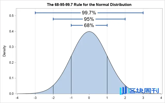
• A. Core Assumptions and Volatility Calculation Assuming that market prices follow a normal distribution in the short term, with a sampling period of 1 second, we examine the sample data from the past 60 seconds. The calculated standard deviation of the marked price relative to the average midpoint in this sample is (σ) of $0.4. This means that, approximately 68% of the time, the price in the next second will fall within the range of [Mean - $0.4, Mean + $0.4].

Source: Idrees

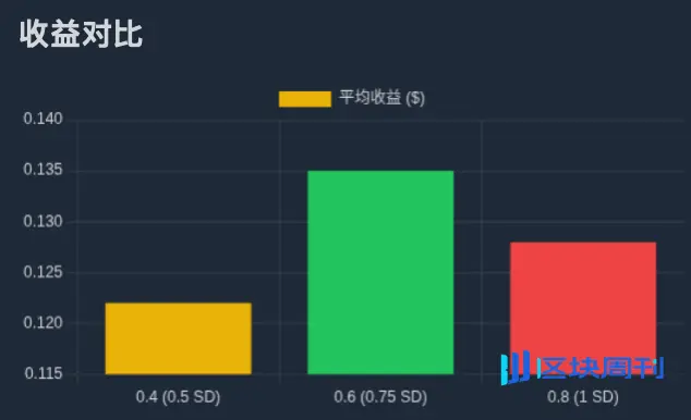
• B. The relationship between spread, probability, and expected return Based on this, we can infer the probability of different spreads being executed and calculate their expected return. For example, if a spread of $0.8 is set (i.e., placing orders of $0.4 on either side of the mean), the price must fluctuate at least one standard deviation to reach the order, which has a probability of about 32%. Assuming each execution can capture half of the spread ($0.4), the expected return per time period is approximately $0.128 (32% × $0.4).

Source: Zhihu

• C. Finding the Optimal Solution Through iterative calculations of different price spreads, it can be found that: with a price spread of $0.2, the expected return is about $0.08; with a price spread of $0.4, the expected return is about $0.122; with a price spread of $0.6, the expected return is about $0.135; with a price spread of $0.8, the expected return is about $0.128. The conclusion is that under this model, the optimal price spread is $0.6, which means placing an order at a position approximately 0.75σ( away from the average price of $0.3 ) can maximize expected returns.

Source: Movemaker

3.5 From Static Models to Dynamic Reality: Multi-Time Frame Risk Management

The fatal flaw of the above model is the assumption of a constant mean. In real markets, the price mean drifts over time. Therefore, professional market makers must adopt a multi-timeframe hierarchical strategy to manage risk.

The core of the strategy lies in using a quantitative model to set the optimal price spread at the micro level (second level), while monitoring the drift of price averages and changes in volatility structure at the meso level (minute level) and macro level (hourly/daily level). When the average deviates, the system dynamically recalibrates the midpoint of the entire quoting range and adjusts inventory positions accordingly.

This layered model ultimately leads to a set of dynamic risk control rules:

1. Automatically widen the spread when the volatility increases on a second-by-second basis.
2. When the medium-term volatility increases, reduce the size of individual orders, but increase the levels of orders, distributing the inventory across a wider price range.
3. When the long-term trend is contrary to the direction of the inventory position, proactive intervention, such as further reducing the size of pending orders or even suspending the strategy, should be taken to prevent systemic risks.

Risk Response Mechanism and Advanced Strategies

4.1 Inventory Risk Management in High-Frequency Market Making

The dynamic strategy model mentioned above falls within the category of high-frequency market making. The core objective of such strategies is to maximize expected profits by setting optimal buy and sell quotes through algorithms, while precisely managing inventory risk.

Inventory risk is defined as the risk that market makers are exposed to adverse price fluctuations due to holding net long or net short positions. When market makers hold long inventory, they face the risk of losses due to falling prices; conversely, when holding short inventory, they face the risk of losses due to rising prices. Effectively managing this risk is key to the long-term survival of market makers.

Professional quantitative models, such as the classic Stoikov model (Stoikov Model), provide us with a mathematical framework to understand its risk management logic. This model is designed to actively manage inventory risk by calculating a dynamically adjusted “reference price.” The bid and ask quotes of market makers will revolve around this new reference price, rather than a static market midpoint. Its core formula is as follows:

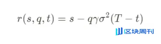
The meanings of each parameter are as follows:

• r(s,q,t): The dynamically adjusted reference price, which serves as the benchmark midpoint for market maker quotations.
• s: Current market midpoint price.
• q: The current inventory level. Positive if long, negative if short.
• γ: Risk aversion parameter. This is a key variable set by market makers that reflects their current risk preference.
• σ: The volatility of the asset.
• (T−t): Time remaining until the end of the trading cycle.

The core idea of the model is that when the inventory of the market maker (q) deviates from its target (usually zero), the model systematically adjusts the mid-price of quotes to incentivize market transactions that bring its inventory back to equilibrium. For example, when holding a long inventory (q>0), the calculated r(s,q,t) will be lower than the market midpoint s, which means the market maker will lower its buy and sell quotes overall, making sell orders more attractive and buy orders less attractive, thereby increasing the probability of liquidating the long inventory.

4.2 Risk Avoidance Parameters (γ) and the Final Choice of Strategy

The risk aversion parameter γ acts as the “regulating valve” for the entire risk management system. Market makers will dynamically adjust the value of γ based on a comprehensive assessment of market conditions (such as expected volatility, macro events, etc.). In stable market conditions, γ may be lower, with strategies leaning towards aggressively capturing spreads; when market risks intensify, γ will be increased, making the strategy extremely conservative, with quotes significantly deviating from the midpoint to quickly reduce risk exposure.

In extreme cases, when the market shows the highest level of risk signals (e.g., liquidity exhaustion, severe price decoupling), the value of γ can become extremely large. At this time, the optimal strategy calculated by the model may be to generate a quote that is extremely deviated from the market and almost impossible to execute. In practice, this is equivalent to a rational decision—temporarily and completely withdrawing liquidity to avoid catastrophic losses due to uncontrollable inventory risks.

4.3 Complex Strategies in Reality

Finally, it must be emphasized that the model discussed in this article is merely an explanation of the core logic of market makers under simplified assumptions. In real, highly competitive market environments, top market makers employ far more complex and multi-layered strategy combinations to maximize profits and manage risks.

These advanced strategies include but are not limited to:

• Hedging Strategy: Market makers typically do not allow their spot inventory to be exposed to risk, but instead establish opposite positions in the derivatives markets such as perpetual contracts, futures, or options to achieve delta neutrality or more complex risk exposure management, converting their risks from price direction risk to other controllable risk factors.
• Special Execution: In certain specific scenarios, the role of market makers can go beyond merely providing passive liquidity. For example, after the project's TGE, they sell a large number of tokens over a certain period using strategies such as TWAP ( time-weighted average price ) or VWAP ( volume-weighted average price ), which constitutes an important source of their profits.

1011 Review: Risk Triggers and the Inevitable Choices of Market Makers

Based on the analytical framework established earlier, we can now review the market upheaval of 1011. When prices exhibit a drastic one-way movement, the internal risk management system of market makers is inevitably triggered. The triggering of this system may be due to a combination of multiple factors: the average loss within a certain time frame exceeds the preset threshold; net inventory positions are rapidly “filled” by counterparties in the market; or after reaching the maximum inventory limit, positions cannot be effectively cleared, leading the system to automatically execute a position contraction procedure.

5.1 Data Analysis: Structural Collapse of the Order Book

To understand the real situation of the market at that time, we must analyze the microstructure of the order book in depth. The following chart, sourced from an order book visualization tool, provides us with evidence:

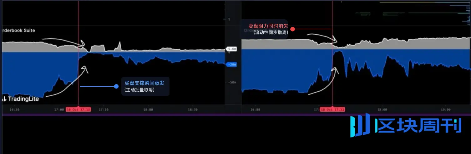
Source: @LisaLewis469193

( Note: To maintain the rigor of the analysis, please consider this chart as a typical representation of the market situation at that time )

This chart intuitively shows the changes in order book depth over time:

• Gray area: Represents the selling liquidity, which is the total of limit orders waiting to sell that are placed above the current price.
• Blue/Black Area: Represents the buy order liquidity, namely the total of limit orders waiting to buy below the current price.

At the precise moment marked by the red vertical line in the image, 5:13 AM, we can observe two unusual phenomena occurring simultaneously:

1. Instant evaporation of buy support: A huge, almost vertical “cliff” has appeared in the blue area at the bottom of the chart. This pattern is completely different from the situation where buy orders are consumed by a large number of transactions— the latter should show a gradual erosion of liquidity in a stepwise manner. The only reasonable explanation for this neat and uniform vertical disappearance is that a large number of limit buy orders were actively, simultaneously, and in bulk canceled.
2. The synchronous disappearance of selling pressure resistance: The gray area at the top of the chart also shows a nearly identical “cliff.” A large number of limit sell orders were actively withdrawn at the same moment.

This series of actions is referred to as “liquidity withdrawal” in trading terminology. It signifies that the main liquidity providers in the market (primarily market makers) have withdrawn their bid-ask quotes almost simultaneously within a very short period, instantly transforming a seemingly liquid market into an extremely fragile “liquidity vacuum.”

5.2 Two Stages of the Event: From Active Withdrawal to Vacuum Formation

Therefore, the process of the sharp decline of 1011 can be clearly divided into two logically progressive stages:

Phase One: Active, Systematic Risk Avoidance Execution

Before 5:13 AM, the market may still be in a superficial state of stability. But at that moment, a key risk signal was triggered — this could be a sudden macro news event or an on-chain risk model from a core protocol (such as USDe/LSTs) issuing an alert.

After receiving the signal, the algorithmic trading system of top market makers immediately executed the preset “emergency hedging procedure.” The goal of this procedure is singular: to minimize its market risk exposure in the shortest possible time, prioritizing this over any profit objectives.

• Why cancel a buy order? This is the most critical defensive operation. The market maker's system predicts that an unprecedented wave of selling pressure is about to arrive. If they do not immediately withdraw their buy orders, these orders will become the “first line of defense” in the market, forced to absorb a large amount of assets that are about to plummet, leading to catastrophic inventory losses.
• Why cancel sell orders simultaneously? This is also based on strict risk control principles. In an environment where volatility is about to sharply increase, keeping sell orders also carries risks (for example, the price may experience a brief upward “false breakout” before a sharp drop, causing sell orders to be executed prematurely at unfavorable prices). Under an institutional-level risk management framework, the safest and most rational choice is to “clear all quotes and enter observation mode” until the market re-emerges with predictability, and then redeploy strategies based on the new market conditions.

Phase Two: The Formation of Liquidity Vacuum and the Free Fall of Prices

After 5:13 AM, with the formation of the “cliff” in the order book, the market structure underwent a fundamental qualitative change, entering what we describe as a “liquidity vacuum” state.

Before actively withdrawing, a large number of sell orders may be needed to consume the stacked buy orders in order to make the market price drop by 1%. However, after the withdrawal, since the support structure below no longer exists, only a very small number of sell orders may be required to cause an equal or even more severe price impact.

Conclusion

The epic market crash of 1011, its direct catalysts and amplifiers, is revealed in the charts as a large-scale, synchronized proactive liquidity withdrawal executed by top market makers. They are neither the “culprits” nor the instigators of the crash, but they are the most efficient “executors” and “amplifiers” of the crash. Through rational, self-preserving collective actions, they created an extremely fragile “liquidity vacuum,” providing perfect conditions for subsequent panic selling, protocol decoupling pressures, and ultimately a chain liquidation of centralized exchanges.